spectrum guide
This notebook shows how to load and perform basic operations on an observed spectrum or set of spectra.
Load the necessary modules.
[1]:
import os
import numpy as np
import pandas as pd
import matplotlib.pyplot as plt
import colorcet as cc
import cmocean as cmo

# from popurri import spectrograph as spc
from popurri import spectrum
from popurri import plotutils

# mpl.rcdefaults()
plotutils.mpl_custom_basic()
plotutils.mpl_size_same(font_size=18)

# Testing
%load_ext autoreload
%autoreload 2
Outputs will be saved here:
[2]:
dirout = './spectrum/'
Single observation: Spectrum class
Here we load a single spectrum observed with CARMENES VIS. To do that we use the class Spectrum from the popurri module spectrum. The only mandatory inputs for Spectrum are the FITS file that contains the spectrum and the corresponding instrument.
[8]:
filin = '/Users/marina/work/data/carmenes_gto/caracal/CARM_VIS/J07446+035/car-20160327T21h25m39s-sci-gtoc-vis_A.fits'  # FITS file with the spectrum
inst = 'carmvis'  # Instrument

# Read spectrum from filin
spec = spectrum.Spectrum(filin, inst, dirout=dirout)

# Spectrum object attributes
# vars(spec)  # print attribute name and value
spec.__dict__.keys()  # print attribute name
[8]:
dict_keys(['filin', 'filname', 'inst', 'obj', 'tag', 'dirout', 'dataspec', 'Spectrograph', 'ords_real', 'ord_ref', 'pixel_ms', 'nord', 'ords', 'npix', 'header', 'dataheader', 'dataord'])
The spectrum data is saved in the attribute dataspec, which is a dictionary containing the data of the FITS file. The main keys are the wavelength w and flux f, containing the wavelengths and fluxes of each order, respectively.
[4]:
# Show the different keys in the dataspec dictionary
print(spec.dataspec.keys())
dict_keys(['w', 'f', 'fe', 'c', 'pix', 'b', 'm', 'w1d', 'f1d', 'fe1d', 'b1d', 'm1d'])
[43]:
# Print shape of the wavelength and flux arrays
print(spec.dataspec['w'].shape)  # nord x npix
print(spec.dataspec['f'].shape)  # nord x npix

# Print wavelength and flux of order 30
print(spec.dataspec['w'][30])
print(spec.dataspec['f'][30])

# Plot the spectrum of order 30
fig, ax = plt.subplots(constrained_layout=True, figsize=(10, 6))
ax.plot(spec.dataspec['w'][30], spec.dataspec['f'][30])
ax.set(xlabel='Wavelength [$\mathrm{\AA}$]', ylabel='Flux', title='Order 30')
plt.show(), plt.close()
(61, 4096)
(61, 4096)
[6887.86217109 6887.8988148  6887.93556006 ... 7007.56148622 7007.5830226
 7007.60455515]
[0.05948321 0.05430395 0.05918692 ... 0.10685489 0.11087142 0.11333495]

[43]:
(None, None)
Plot the spectrum
The Spectrum class comes with a few functions to easily plot the data.
Plot all orders using fig_spectrum:
[6]:
# By default orders are plotted following the default color cycle
spec.fig_spectrum(title='All orders', sh=True, sv=False)

We can also specify a single order with the parameter ords:
[44]:
# Plot 25 (for CARMENES VIS this one contains Halpha)
spec.fig_spectrum(ords=spec.ords[25], title='Order 25', sh=True, sv=False)

Or a set of specific orders:
[9]:
# Plott odd/even orders with different alpha
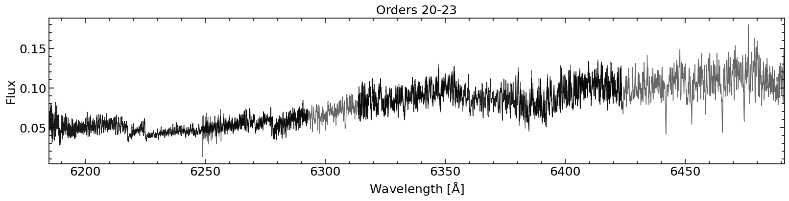
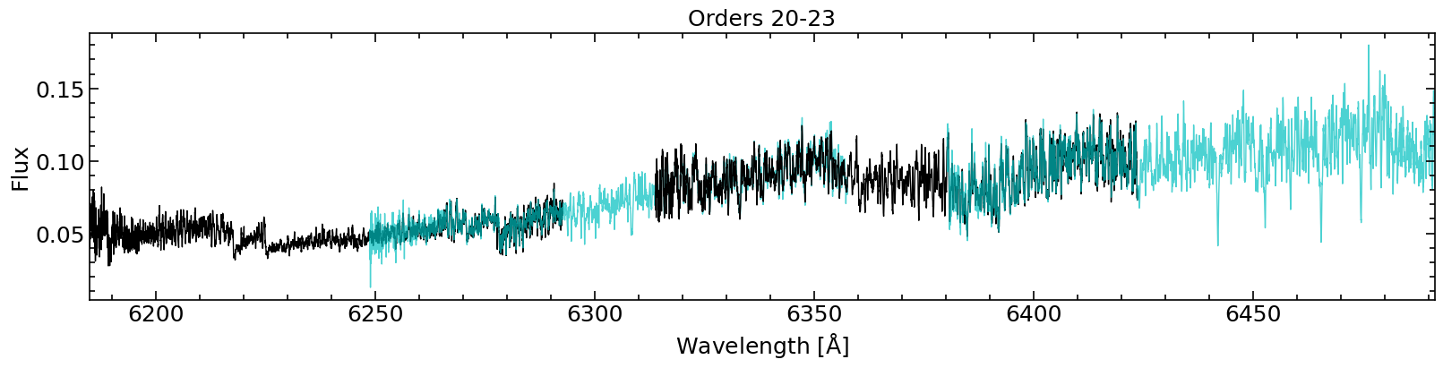
spec.fig_spectrum(ords=spec.ords[20:24], title='Orders 20-23', color='k', alpha=0.9, alphaother=0.6, sh=True, sv=False)
# Plott odd/even orders with different colors
spec.fig_spectrum(ords=spec.ords[20:24], title='Orders 20-23', color='k', colorother='c', sh=True, sv=False)
We can also plot a specific wavelength range with the paramters wmin and wmax:
[46]:
spec.fig_spectrum(wmin=7550, wmax=7575, title='Wavelength range 7550-7575 $[\mathrm{\AA}]$', sh=True, sv=False, lw=2)

All the orders covered by the wavelength range specified are plotted:
[48]:
spec.fig_spectrum(wmin=7550, wmax=7595, title='Wavelength range 7550-7575 $[\mathrm{\AA}]$', sh=True, sv=False)

The method fig_spectrum actually calls another method called plot_spectrum, which we can use to access the “axes”, and not only the final “figure”. This can be useful to e.g. plot 2 orders on different panels:
[10]:
fig, ax = plt.subplots(2, 1, figsize=(16, 8), constrained_layout=True)
ax[0] = spec.plot_spectrum(ax=ax[0], ords=[20], legend=True, legendloc='upper left', xlabel='')
ax[1] = spec.plot_spectrum(ax=ax[1], ords=[21], legend=True, legendloc='upper left')
plt.suptitle(spec.filname)
plt.show(), plt.close()

[10]:
(None, None)
We can also specify a colormap with cmap:
[11]:
spec.fig_spectrum(ords=spec.ords[26:54], title='Orders 26-53, colormap', cmap=cc.cm.rainbow4, sh=True, sv=False)

We can also plot in units of pixel instead of wavelengths. The orders will appear on top of each other then:
[12]:
# Plot pixel instead of wavelength -> Orders on top of each other
spec.fig_spectrum(figsize=(8, 4), x='pix', ords=spec.ords[26:54], title='Orders 26-53', xlabel='Pixel', ylabel='Norm. flux + offset', cmap=cc.cm.rainbow4, sh=True, sv=False)

To avoid this happening, we can normalise the flux of each order with e.g. normflux=np.nanmax and shift (offset) it with e.g. offset=1:
[13]:
spec.fig_spectrum(figsize=(8, 10), x='pix', normflux=np.nanmax, offset=1, ords=spec.ords[26:54], title='Orders 26-53', xlabel='Pixel', ylabel='Norm. flux + offset', cmap=cc.cm.rainbow4, sh=True, sv=False)
(61, 4096) (61, 4096)

Instead doing the above with fig_spectrum, we can directly use fig_spectrum_pix (and plot_spectrum_pix), which has parameters pre-defined to plot with pixel in the x-axis, flux normalised and shifted.
[14]:
spec.fig_spectrum_pix(figsize=(8, 10), ords=spec.ords[26:54], title='Orders 26-53', cmap=cc.cm.rainbow4, sh=True, sv=False)
(61, 4096) (61, 4096)

The normalisation function can be set to something different than the maximum with normflux. The offset can also be changed with offset. Note that if we plot all orders, not all of them will look good if there are noisy pixels or strong emission lines:
[15]:
spec.fig_spectrum_pix(ords=spec.ords[26:54], normflux=np.nanmedian, cmap=cc.cm.rainbow4, title='Orders 26-53, median normalisation', sh=True, sv=False)
spec.fig_spectrum_pix(normflux=np.nanmedian, cmap=cc.cm.rainbow4, title='All orders, median normalisation', sh=True, sv=False)
(61, 4096) (61, 4096)

(61, 4096) (61, 4096)

Plot order data
We can plot properties like the signal-to-noise ratio (S/N) of each order with the method fig_dataord, which uses the data from Spectrum.dataord:
[16]:
spec.fig_dataord('snr', z='snr', ylabel='S/N', zlabel='S/N', title=spec.filname, cmap='plasma', sh=True, sv=False)

As with fig_spectrum and plot_spectrum, there is also the function plot_dataord to directly access the “axes”.
Single observation CARMENES NIR
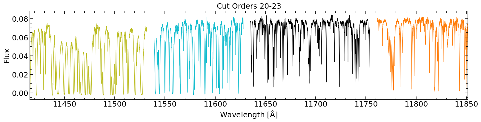
Read a CARMENES NIR ('carmnir') observation. Note: Orders can be split into the two detectors (ordcut).
[50]:
# Observation
inst = 'carmnir'
filin = '/Users/marina/work/data/carmenes_gto/caracal/CARM_NIR/J07446+035/car-20160924T05h04m12s-sci-gtoc-nir_A.fits'

# Read spectrum from filin
spec = spectrum.Spectrum(filin, inst, dirout=dirout, ordcut=True, saveordnoncut=True)
spec_nocut = spectrum.Spectrum(filin, inst, dirout=dirout, ordcut=False, saveordnoncut=False)

# # Spectrum object variables
# vars(spec)
Plot the spectrum.
[51]:
# Plot all orders
fig, ax = plt.subplots(1, 1, figsize=(16, 4), constrained_layout=True)
ax = spec.plot_spectrum(ax=ax, title='All orders')
plt.show()
plt.close()

# Plot some of the central orders
fig, ax = plt.subplots(1, 1, figsize=(16, 4), constrained_layout=True)
ax = spec.plot_spectrum(ax=ax, ords=spec.ords[20:24], title='Orders 20-23')
plt.show()
plt.close()

# Plot the order with Halpha
fig, ax = plt.subplots(1, 1, figsize=(16, 4), constrained_layout=True)
ax = spec.plot_spectrum(ax=ax, ords=spec.ords[25], title='Order 25')
plt.show()
plt.close()

# Plot a specific wavelength range
fig, ax = plt.subplots(1, 1, figsize=(16, 4), constrained_layout=True)
ax = spec.plot_spectrum(ax=ax, wmin=10900, wmax=11500, title='Wavelength range 10900-11500 $[\mathrm{\AA}]$')
plt.show()
plt.close()


Compare spectrum with orders cut and not cut.
[52]:
# Compare orders cut and nocut
print('Orders', spec.ords, 'total number of orders', len(spec.ords))
fig, ax = plt.subplots(1, 1, figsize=(16, 4), constrained_layout=True)
ax = spec.plot_spectrum(ax=ax, ords=spec.ords[20:24], title='Cut Orders 20-23')
plt.show()
plt.close()

print('Orders', spec_nocut.ords, 'total number of orders', len(spec_nocut.ords))
fig, ax = plt.subplots(1, 1, figsize=(16, 4), constrained_layout=True)
ax = spec_nocut.plot_spectrum(ax=ax, ords=spec.ords[10:12], title='No cut Orders 10-12')
plt.show()
plt.close()

fig, ax = plt.subplots(1, 1, figsize=(16, 4), constrained_layout=True)
ax = spec.plot_spectrum(ax=ax, ords=spec.ords[20:24], lw=3, alpha=0.5, zorder=2)
ax = spec_nocut.plot_spectrum(ax=ax, ords=spec.ords[10:12], lw=3, linestyle=':', alpha=0.5, zorder=1)
plt.show()
plt.close()
Orders [ 0  1  2  3  4  5  6  7  8  9 10 11 12 13 14 15 16 17 18 19 20 21 22 23
 24 25 26 27 28 29 30 31 32 33 34 35 36 37 38 39 40 41 42 43 44 45 46 47
 48 49 50 51 52 53 54 55] total number of orders 56
Orders [ 0  1  2  3  4  5  6  7  8  9 10 11 12 13 14 15 16 17 18 19 20 21 22 23
 24 25 26 27] total number of orders 28


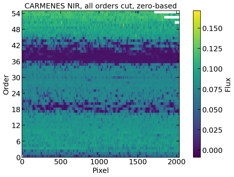
Plot order map, compare cut and no cut (no cut has less orders).
Note that for the cut case, if we use the real order indexing, the y-axis is not correct (because 2 different cut orders have the same real index).
[20]:
# Map of all orders flux
spec_nocut.fig_spectrum_map(title='CARMENES NIR, all orders no-cut, zero-based', sh=True, sv=False)

spec_nocut.fig_spectrum_map(ordtype='real', title='CARMENES NIR, all orders no-cut, real', sh=True, sv=False)

spec.fig_spectrum_map(title='CARMENES NIR, all orders cut, zero-based', sh=True, sv=False)

spec.fig_spectrum_map(ordtype='real', title='CARMENES NIR, all orders cut, real\nNote that there are 2 "orders" per real index,\ni.e. the y-axis labels are not correct!', sh=True, sv=False)


Plot orders map, cut in flux
[21]:
# Map of all orders flux, real orders, and cut in flux
spec.fig_spectrum_map(ordtype='real', vmin=0, vmax=0.1, title='CARMENES NIR, all orders cut, real', sh=True, sv=False)

spec.fig_spectrum_map(ordtype='zero', vmax=0.05, title='CARMENES NIR, all orders cut, zero-based', sh=True, sv=False)

spec.fig_spectrum_map(ordtype='zero', vmin=0, title='CARMENES NIR, all orders cut, zero-based', sh=True, sv=False)


Plot orders map, cut orders.
[22]:
# Map of some orders
spec.fig_spectrum_map(ords=np.arange(4, 14, 1), ordtype='zero', cmap='gray', sh=True, sv=False)
spec_nocut.fig_spectrum_map(ords=np.arange(4, 8, 1), ordtype='real', cmap='gray', sh=True, sv=False)
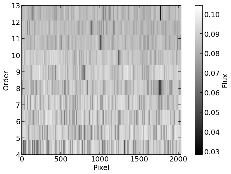

Plot orders map, cut orders and pixels
[23]:
# Map of some pixels
spec.fig_spectrum_map(ords=np.arange(4, 24, 1), ordtype='zero', title='Full', sh=True, sv=False)
spec.fig_spectrum_map(ords=np.arange(4, 24, 1), pixs=np.arange(300, 325, 1), ordtype='zero', title='Cut', sh=True, sv=False)


List of observations: Spectra class
CARMENES VIS
[9]:
lisfil = [
    '/Users/marina/work/data/carmenes_gto/caracal/CARM_VIS/J07446+035/car-20160318T22h26m50s-sci-gtoc-vis_A.fits',
    '/Users/marina/work/data/carmenes_gto/caracal/CARM_VIS/J07446+035/car-20160327T21h25m39s-sci-gtoc-vis_A.fits',
    '/Users/marina/work/data/carmenes_gto/caracal/CARM_VIS/J07446+035/car-20160411T20h12m48s-sci-gtoc-vis_A.fits',
    '/Users/marina/work/data/carmenes_gto/caracal/CARM_VIS/J07446+035/car-20170109T02h38m37s-sci-gtoc-vis_A.fits',
    '/Users/marina/work/data/carmenes_gto/caracal/CARM_VIS/J07446+035/car-20170302T20h25m06s-sci-gtoc-vis_A.fits',
    '/Users/marina/work/data/carmenes_gto/caracal/CARM_VIS/J07446+035/car-20170412T20h02m25s-sci-gtoc-vis_A.fits',
    '/Users/marina/work/data/carmenes_gto/caracal/CARM_VIS/J07446+035/car-20171230T01h42m48s-sci-gtoc-vis_A.fits',
    '/Users/marina/work/data/carmenes_gto/caracal/CARM_VIS/J07446+035/car-20180102T01h14m44s-sci-gtoc-vis_A.fits',
]
inst = 'carmvis'

# Read spectrum from filin
lisspec = spectrum.Spectra(lisfil, inst, dirout=dirout)

# vars(lisspec)
++++++ dict_keys(['airhum', 'airmass', 'airmass_end', 'airmass_start', 'berv', 'berv_max', 'bjd', 'date_start', 'dec_deg', 'drift', 'drift_err', 'exptime', 'fibers', 'gain', 'hjd', 'iwp', 'iwp_end', 'iwv_start', 'jd', 'mjd', 'mjd_start', 'moondist', 'obj', 'pi', 'program', 'ra_deg', 'ra_h', 'radecsys', 'red_pipeline_version', 'ron', 'seeing', 'seeing_end', 'seeing_start', 'snr_oref', 'telescope', 'snro0', 'snro1', 'snro2', 'snro3', 'snro4', 'snro5', 'snro6', 'snro7', 'snro8', 'snro9', 'snro10', 'snro11', 'snro12', 'snro13', 'snro14', 'snro15', 'snro16', 'snro17', 'snro18', 'snro19', 'snro20', 'snro21', 'snro22', 'snro23', 'snro24', 'snro25', 'snro26', 'snro27', 'snro28', 'snro29', 'snro30', 'snro31', 'snro32', 'snro33', 'snro34', 'snro35', 'snro36', 'snro37', 'snro38', 'snro39', 'snro40', 'snro41', 'snro42', 'snro43', 'snro44', 'snro45', 'snro46', 'snro47', 'snro48', 'snro49', 'snro50', 'snro51', 'snro52', 'snro53', 'snro54', 'snro55', 'snro56', 'snro57', 'snro58', 'snro59', 'snro60'])
++++++ Index(['snro0', 'snro1', 'snro2', 'snro3', 'snro4', 'snro5', 'snro6', 'snro7',
       'snro8', 'snro9', 'snro10', 'snro11', 'snro12', 'snro13', 'snro14',
       'snro15', 'snro16', 'snro17', 'snro18', 'snro19', 'snro20', 'snro21',
       'snro22', 'snro23', 'snro24', 'snro25', 'snro26', 'snro27', 'snro28',
       'snro29', 'snro30', 'snro31', 'snro32', 'snro33', 'snro34', 'snro35',
       'snro36', 'snro37', 'snro38', 'snro39', 'snro40', 'snro41', 'snro42',
       'snro43', 'snro44', 'snro45', 'snro46', 'snro47', 'snro48', 'snro49',
       'snro50', 'snro51', 'snro52', 'snro53', 'snro54', 'snro55', 'snro56',
       'snro57', 'snro58', 'snro59', 'snro60'],
      dtype='object')
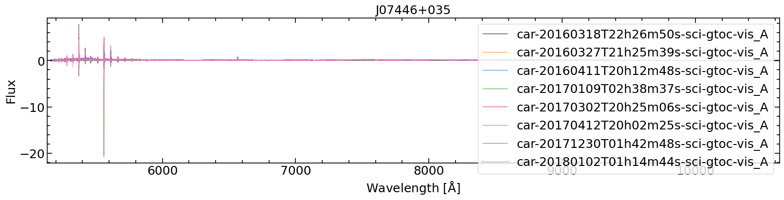
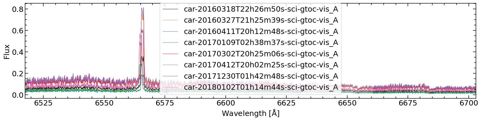
Plot spectrum of all observations
[55]:
# All orders
lisspec.fig_spectra(legendwhich='all', legendlabel='obs', sh=True, sv=False, title=lisspec.obj)
# Specific orders `ords`
lisspec.fig_spectra(ords=[25, 26], legendwhich='all', legendlabel='obs', sh=True, sv=False)
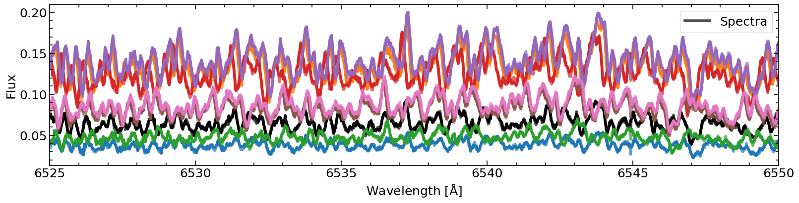
# Specific wavelength range `wmin` and `wmax` (must be within the range of the orders in `ords`, if not nothing will be plotted)
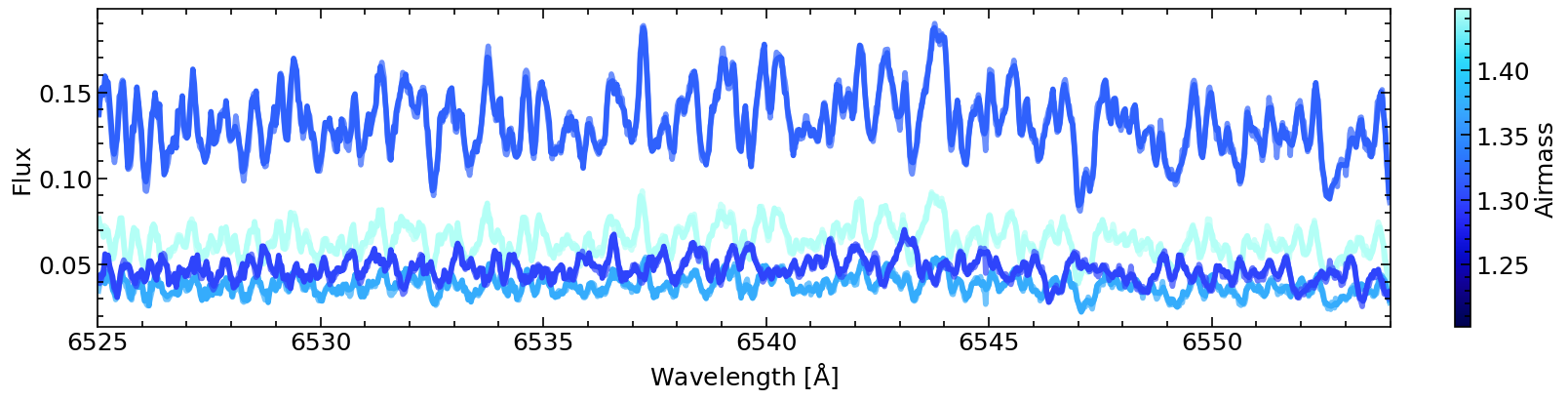
lisspec.fig_spectra(ords=[25, 26], wmin=6525, wmax=6550, legendwhich='all', legendlabel='obs', sh=True, sv=False, lw=4)
# Without specifing the orders
lisspec.fig_spectra(wmin=6525, wmax=6550, legendwhich='first', legendlabel='Spectra', sh=True, sv=False, lw=4)
/Users/marina/anaconda3/envs/popurri/lib/python3.11/site-packages/IPython/core/pylabtools.py:152: UserWarning: Creating legend with loc="best" can be slow with large amounts of data.
  fig.canvas.print_figure(bytes_io, **kw)

[57]:
# Plot all observations with colormap of airmass
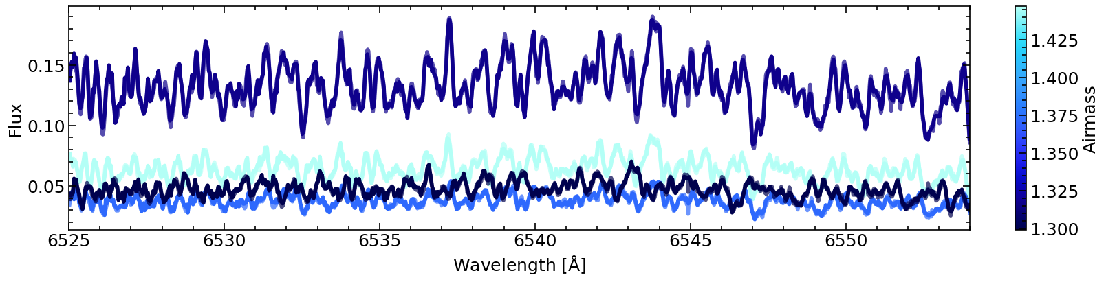
lisspec.fig_spectra(ords=[25, 26], wmin=6525, wmax=6554, sh=True, sv=False, cmap=cc.cm.kbc, lw=4, cprop=lisspec.dataheader['airmass'], cbarlabel='Airmass')
# Subset of observations, keep colormap of all observations
lisspec.fig_spectra(ords=[25, 26], wmin=6525, wmax=6554, sh=True, sv=False, cmap=cc.cm.kbc, lw=4, cprop=lisspec.dataheader['airmass'], cbarlabel='Airmass', lisspec=[0, 2, 3, 5], cprop_all=True)
# Subset of observations, update colormap to only the subset
lisspec.fig_spectra(ords=[25, 26], wmin=6525, wmax=6554, sh=True, sv=False, cmap=cc.cm.kbc, lw=4, cprop=lisspec.dataheader['airmass'], cbarlabel='Airmass', lisspec=[0, 2, 3, 5])

Plot per order property of all observations
[27]:
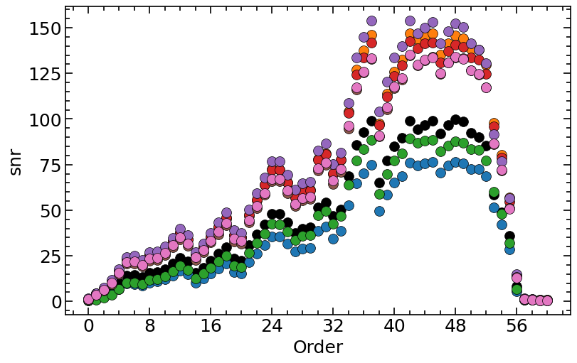
# Plot S/N per order, for all observations
lisspec.fig_dataord('snr', sh=True, sv=False)

# Color from colormap (following observation index)
lisspec.fig_dataord('snr', ylabel='S/N', cmap='plasma', sh=True, sv=False)

# Color from colormap following property bjd in `dataheader` (should be the similar colors as above if observations are ordered in time, difference due to difference in spacing between index and BJD)
lisspec.fig_dataord('snr', ylabel='S/N', z='bjd', zlabel='BJD', cmap='plasma', sh=True, sv=False)

# Color from colormap following property airmass in `dataheader`
lisspec.fig_dataord('snr', ylabel='S/N', z='airmass', zlabel='Airmass', cmap=cc.cm.kbc, alpha=0.9, sh=True, sv=False)
/Users/marina/work/code/popurri/popurri/spectrum.py:1272: UserWarning: *c* argument looks like a single numeric RGB or RGBA sequence, which should be avoided as value-mapping will have precedence in case its length matches with *x* & *y*.  Please use the *color* keyword-argument or provide a 2D array with a single row if you intend to specify the same RGB or RGBA value for all points.
  sc = ax.scatter(ords, datay.iloc[i], c=c, zorder=zorder, s=s, edgecolors=edgecolors, linewidths=linewidths, **kwargs)


S/N
[28]:
lisfil = [
    '/Users/marina/work/data/carmenes_gto/caracal/CARM_VIS/J07446+035/car-20160318T22h26m50s-sci-gtoc-vis_A.fits',
    '/Users/marina/work/data/carmenes_gto/caracal/CARM_VIS/J07446+035/car-20160327T21h25m39s-sci-gtoc-vis_A.fits',
    '/Users/marina/work/data/carmenes_gto/caracal/CARM_VIS/J07446+035/car-20160411T20h12m48s-sci-gtoc-vis_A.fits',
    '/Users/marina/work/data/carmenes_gto/caracal/CARM_VIS/J07446+035/car-20170109T02h38m37s-sci-gtoc-vis_A.fits',
    '/Users/marina/work/data/carmenes_gto/caracal/CARM_VIS/J07446+035/car-20170302T20h25m06s-sci-gtoc-vis_A.fits',
    '/Users/marina/work/data/carmenes_gto/caracal/CARM_VIS/J07446+035/car-20170412T20h02m25s-sci-gtoc-vis_A.fits',
    '/Users/marina/work/data/carmenes_gto/caracal/CARM_VIS/J07446+035/car-20171230T01h42m48s-sci-gtoc-vis_A.fits',
    '/Users/marina/work/data/carmenes_gto/caracal/CARM_VIS/J07446+035/car-20180102T01h14m44s-sci-gtoc-vis_A.fits',
]
inst = 'carmvis'

# Read spectrum from filin
lisspec = spectrum.Spectra(lisfil, inst, dirout=dirout)

# vars(lisspec)
[29]:
lisspec.dataheader
[29]:
| airhum | airmass | airmass_end | airmass_start | berv | berv_max | bjd | date_start | dec_deg | drift | ... | snro51 | snro52 | snro53 | snro54 | snro55 | snro56 | snro57 | snro58 | snro59 | snro60 | |
|---|---|---|---|---|---|---|---|---|---|---|---|---|---|---|---|---|---|---|---|---|---|
| car-20160318T22h26m50s-sci-gtoc-vis_A | NaN | 1.4472 | NaN | NaN | -24.960843 | NaN | 57466.441682 | 2016-03-18T22:26:50 | 3.550333 | 5.280760 | ... | 89.960 | 85.466 | 58.368 | 48.723 | 36.025 | 8.4427 | 0.88638 | 0.76074 | 0.68711 | 0.63991 |
| car-20160327T21h25m39s-sci-gtoc-vis_A | NaN | 1.3556 | NaN | NaN | -26.745976 | NaN | 57475.400098 | 2016-03-27T21:25:39 | 3.550333 | 8.804540 | ... | 137.750 | 129.760 | 97.864 | 80.232 | 56.793 | 14.5830 | 1.31660 | 1.11120 | 0.79862 | 0.71682 |
| car-20160411T20h12m48s-sci-gtoc-vis_A | NaN | 1.3172 | NaN | NaN | -28.345505 | NaN | 57490.349229 | 2016-04-11T20:12:48 | 3.550333 | 2.437240 | ... | 72.699 | 68.544 | 51.685 | 42.036 | 28.376 | 5.6667 | 0.86901 | 0.79521 | 0.70693 | 0.62124 |
| car-20170109T02h38m37s-sci-gtoc-vis_A | NaN | 1.3719 | NaN | NaN | 4.224916 | NaN | 57762.616890 | 2017-01-09T02:38:37 | 3.550389 | 4.998870 | ... | 83.165 | 77.302 | 59.964 | 48.169 | 31.995 | 6.6406 | 1.03250 | 0.71653 | 0.61393 | 0.66281 |
| car-20170302T20h25m06s-sci-gtoc-vis_A | NaN | 1.2270 | NaN | NaN | -19.819234 | NaN | 57815.357620 | 2017-03-02T20:25:06 | 3.550389 | -0.789388 | ... | 132.670 | 124.770 | 95.966 | 78.689 | 54.534 | 14.2390 | 1.30630 | 1.06210 | 0.82434 | 0.75072 |
| car-20170412T20h02m25s-sci-gtoc-vis_A | NaN | 1.2993 | NaN | NaN | -28.340839 | NaN | 57856.339926 | 2017-04-12T20:02:25 | 3.550389 | -7.596280 | ... | 138.030 | 130.470 | 91.573 | 76.745 | 56.420 | 14.8890 | 1.70510 | 1.34840 | 0.80956 | 0.71723 |
| car-20171230T01h42m48s-sci-gtoc-vis_A | NaN | 1.2070 | NaN | NaN | 9.407480 | NaN | 58117.580624 | 2017-12-30T01:42:48 | 3.550389 | 2.974620 | ... | 124.200 | 117.330 | 86.239 | 71.868 | 51.068 | 13.2280 | 1.25430 | 0.99787 | 0.75848 | 0.72809 |
| car-20180102T01h14m44s-sci-gtoc-vis_A | NaN | 1.2022 | NaN | NaN | 8.004895 | NaN | 58120.561319 | 2018-01-02T01:14:44 | 3.550389 | 4.125970 | ... | 124.850 | 117.390 | 86.493 | 72.102 | 50.707 | 13.0370 | 1.15830 | 1.00020 | 0.58225 | 0.55213 |
8 rows × 157 columns
[30]:
lisspec.dataord['snr']
[30]:
| 0 | 1 | 2 | 3 | 4 | 5 | 6 | 7 | 8 | 9 | ... | 51 | 52 | 53 | 54 | 55 | 56 | 57 | 58 | 59 | 60 | |
|---|---|---|---|---|---|---|---|---|---|---|---|---|---|---|---|---|---|---|---|---|---|
| car-20160318T22h26m50s-sci-gtoc-vis_A | 0.73764 | 2.1662 | 3.9004 | 6.2601 | 10.2700 | 14.1330 | 14.5690 | 13.2800 | 15.776 | 16.165 | ... | 89.960 | 85.466 | 58.368 | 48.723 | 36.025 | 8.4427 | 0.88638 | 0.76074 | 0.68711 | 0.63991 |
| car-20160327T21h25m39s-sci-gtoc-vis_A | 1.31520 | 4.3115 | 7.0373 | 11.3970 | 17.3990 | 23.2760 | 23.3070 | 21.6080 | 25.449 | 25.834 | ... | 137.750 | 129.760 | 97.864 | 80.232 | 56.793 | 14.5830 | 1.31660 | 1.11120 | 0.79862 | 0.71682 |
| car-20160411T20h12m48s-sci-gtoc-vis_A | 0.63032 | 1.2139 | 2.5354 | 4.0185 | 6.5503 | 9.6718 | 9.6223 | 8.6419 | 10.409 | 10.867 | ... | 72.699 | 68.544 | 51.685 | 42.036 | 28.376 | 5.6667 | 0.86901 | 0.79521 | 0.70693 | 0.62124 |
| car-20170109T02h38m37s-sci-gtoc-vis_A | 0.58134 | 1.0072 | 2.0739 | 3.7211 | 6.5540 | 10.1870 | 10.3310 | 9.4551 | 11.851 | 12.118 | ... | 83.165 | 77.302 | 59.964 | 48.169 | 31.995 | 6.6406 | 1.03250 | 0.71653 | 0.61393 | 0.66281 |
| car-20170302T20h25m06s-sci-gtoc-vis_A | 1.36440 | 4.2096 | 6.8966 | 11.0790 | 16.9610 | 23.4030 | 23.3600 | 21.5520 | 25.536 | 25.226 | ... | 132.670 | 124.770 | 95.966 | 78.689 | 54.534 | 14.2390 | 1.30630 | 1.06210 | 0.82434 | 0.75072 |
| car-20170412T20h02m25s-sci-gtoc-vis_A | 1.54050 | 4.4375 | 7.6438 | 11.8830 | 17.7070 | 24.3340 | 24.9740 | 22.7590 | 26.802 | 27.506 | ... | 138.030 | 130.470 | 91.573 | 76.745 | 56.420 | 14.8890 | 1.70510 | 1.34840 | 0.80956 | 0.71723 |
| car-20171230T01h42m48s-sci-gtoc-vis_A | 1.04680 | 3.4788 | 6.0343 | 9.6238 | 15.0920 | 20.7060 | 20.5970 | 19.0140 | 22.370 | 22.571 | ... | 124.200 | 117.330 | 86.239 | 71.868 | 51.068 | 13.2280 | 1.25430 | 0.99787 | 0.75848 | 0.72809 |
| car-20180102T01h14m44s-sci-gtoc-vis_A | 1.27660 | 3.7896 | 6.4974 | 10.2110 | 15.7960 | 21.5130 | 21.8060 | 19.9950 | 23.623 | 23.680 | ... | 124.850 | 117.390 | 86.493 | 72.102 | 50.707 | 13.0370 | 1.15830 | 1.00020 | 0.58225 | 0.55213 |
8 rows × 61 columns
[31]:
spec.header['*CARACAL FOX SNR*']
[31]:
HIERARCH CARACAL FOX SNR 0 = 27.503 / SNR per pixel in order 63
HIERARCH CARACAL FOX SNR 1 = 44.568 / SNR per pixel in order 62
HIERARCH CARACAL FOX SNR 2 = 49.54 / SNR per pixel in order 61
HIERARCH CARACAL FOX SNR 3 = 53.839 / SNR per pixel in order 60
HIERARCH CARACAL FOX SNR 4 = 56.171 / SNR per pixel in order 59
HIERARCH CARACAL FOX SNR 5 = 60.053 / SNR per pixel in order 58
HIERARCH CARACAL FOX SNR 6 = 61.869 / SNR per pixel in order 57
HIERARCH CARACAL FOX SNR 7 = 64.983 / SNR per pixel in order 56
HIERARCH CARACAL FOX SNR 8 = 63.016 / SNR per pixel in order 55
HIERARCH CARACAL FOX SNR 9 = 42.813 / SNR per pixel in order 54
HIERARCH CARACAL FOX SNR 10 = 50.537 / SNR per pixel in order 53
HIERARCH CARACAL FOX SNR 11 = 69.799 / SNR per pixel in order 52
HIERARCH CARACAL FOX SNR 12 = 72.311 / SNR per pixel in order 51
HIERARCH CARACAL FOX SNR 13 = 75.194 / SNR per pixel in order 50
HIERARCH CARACAL FOX SNR 14 = 76.784 / SNR per pixel in order 49
HIERARCH CARACAL FOX SNR 15 = 74.952 / SNR per pixel in order 48
HIERARCH CARACAL FOX SNR 16 = 80.944 / SNR per pixel in order 47
HIERARCH CARACAL FOX SNR 17 = 76.919 / SNR per pixel in order 46
HIERARCH CARACAL FOX SNR 18 = 7.4168 / SNR per pixel in order 45
HIERARCH CARACAL FOX SNR 19 = 1.9858 / SNR per pixel in order 44
HIERARCH CARACAL FOX SNR 20 = 3.7664 / SNR per pixel in order 43
HIERARCH CARACAL FOX SNR 21 = 40.704 / SNR per pixel in order 42
HIERARCH CARACAL FOX SNR 22 = 59.763 / SNR per pixel in order 41
HIERARCH CARACAL FOX SNR 23 = 79.162 / SNR per pixel in order 40
HIERARCH CARACAL FOX SNR 24 = 82.567 / SNR per pixel in order 39
HIERARCH CARACAL FOX SNR 25 = 83.069 / SNR per pixel in order 38
HIERARCH CARACAL FOX SNR 26 = 81.844 / SNR per pixel in order 37
HIERARCH CARACAL FOX SNR 27 = 75.223 / SNR per pixel in order 36
HIERARCH CARACAL FOX SNR 28 = 34.321 / SNR per pixel in order 63
HIERARCH CARACAL FOX SNR 29 = 42.877 / SNR per pixel in order 62
HIERARCH CARACAL FOX SNR 30 = 47.653 / SNR per pixel in order 61
HIERARCH CARACAL FOX SNR 31 = 50.821 / SNR per pixel in order 60
HIERARCH CARACAL FOX SNR 32 = 53.272 / SNR per pixel in order 59
HIERARCH CARACAL FOX SNR 33 = 53.863 / SNR per pixel in order 58
HIERARCH CARACAL FOX SNR 34 = 55.783 / SNR per pixel in order 57
HIERARCH CARACAL FOX SNR 35 = 57.813 / SNR per pixel in order 56
HIERARCH CARACAL FOX SNR 36 = 41.934 / SNR per pixel in order 55
HIERARCH CARACAL FOX SNR 37 = 39.566 / SNR per pixel in order 54
HIERARCH CARACAL FOX SNR 38 = 52.746 / SNR per pixel in order 53
HIERARCH CARACAL FOX SNR 39 = 59.807 / SNR per pixel in order 52
HIERARCH CARACAL FOX SNR 40 = 61.984 / SNR per pixel in order 51
HIERARCH CARACAL FOX SNR 41 = 67.17 / SNR per pixel in order 50
HIERARCH CARACAL FOX SNR 42 = 66.677 / SNR per pixel in order 49
HIERARCH CARACAL FOX SNR 43 = 68.484 / SNR per pixel in order 48
HIERARCH CARACAL FOX SNR 44 = 68.069 / SNR per pixel in order 47
HIERARCH CARACAL FOX SNR 45 = 55.684 / SNR per pixel in order 46
HIERARCH CARACAL FOX SNR 46 = 2.0268 / SNR per pixel in order 45
HIERARCH CARACAL FOX SNR 47 = 1.8734 / SNR per pixel in order 44
HIERARCH CARACAL FOX SNR 48 = 15.186 / SNR per pixel in order 43
HIERARCH CARACAL FOX SNR 49 = 48.42 / SNR per pixel in order 42
HIERARCH CARACAL FOX SNR 50 = 60.951 / SNR per pixel in order 41
HIERARCH CARACAL FOX SNR 51 = 67.134 / SNR per pixel in order 40
HIERARCH CARACAL FOX SNR 52 = 67.613 / SNR per pixel in order 39
HIERARCH CARACAL FOX SNR 53 = 67.725 / SNR per pixel in order 38
HIERARCH CARACAL FOX SNR 54 = 67.739 / SNR per pixel in order 37
HIERARCH CARACAL FOX SNR 55 = 60.812 / SNR per pixel in order 36
Doppler shift
Default: Doppler shift ‘w’ and save result in ‘wshift’, both in Spectrum.dataspec. Can change these keywords with x='w', xnew='wshift' when calling `dopplershift.
[69]:
# single obs
filin = '/Users/marina/work/data/carmenes_gto/caracal/CARM_VIS/J07446+035/car-20160327T21h25m39s-sci-gtoc-vis_A.fits'
inst = 'carmvis'

# Read spectrum from filin
spec = spectrum.Spectrum(filin, inst, dirout=dirout)

# Doppler shift by BERV
spec.dopplershift(spec.dataheader['berv']*1.e3)  # Shift in m/s
[72]:
print('Original w:', spec.dataspec['w'][20])
print('Doppler shifted w:', spec.dataspec['wshift'][20])

fig, ax = plt.subplots(figsize=(8, 6), constrained_layout=True)
spec.plot_spectrum(ax=ax, wmin=6240, wmax=6245, color='k', lw=2, legendlabel='Original')
spec.plot_spectrum(ax=ax, x='wshift', wmin=6240, wmax=6245, color='r', lw=2, linestyle='dashed', legendlabel=f'Shifted {spec.dataheader["berv"]:.2f} km/s')
ax.legend()
plt.show(), plt.close()
Original w: [6184.96519528 6184.99817627 6185.03124863 ... 6292.63677358 6292.65612866
 6292.67548029]
Doppler shifted w: [6184.41342839 6184.44640643 6184.47947585 ... 6292.0754012  6292.09475455
 6292.11410446]

[72]:
(None, None)
[3]:
# Multiple obs
lisfil = [
    '/Users/marina/work/data/carmenes_gto/caracal/CARM_VIS/J07446+035/car-20160318T22h26m50s-sci-gtoc-vis_A.fits',
    '/Users/marina/work/data/carmenes_gto/caracal/CARM_VIS/J07446+035/car-20160327T21h25m39s-sci-gtoc-vis_A.fits',
    '/Users/marina/work/data/carmenes_gto/caracal/CARM_VIS/J07446+035/car-20160411T20h12m48s-sci-gtoc-vis_A.fits',
    '/Users/marina/work/data/carmenes_gto/caracal/CARM_VIS/J07446+035/car-20170109T02h38m37s-sci-gtoc-vis_A.fits',
    '/Users/marina/work/data/carmenes_gto/caracal/CARM_VIS/J07446+035/car-20170302T20h25m06s-sci-gtoc-vis_A.fits',
    '/Users/marina/work/data/carmenes_gto/caracal/CARM_VIS/J07446+035/car-20170412T20h02m25s-sci-gtoc-vis_A.fits',
    '/Users/marina/work/data/carmenes_gto/caracal/CARM_VIS/J07446+035/car-20171230T01h42m48s-sci-gtoc-vis_A.fits',
    '/Users/marina/work/data/carmenes_gto/caracal/CARM_VIS/J07446+035/car-20180102T01h14m44s-sci-gtoc-vis_A.fits',
]
inst = 'carmvis'

# Read spectrum from filin
lisspec = spectrum.Spectra(lisfil, inst, dirout=dirout)

# Doppler shift by BERV
lisv = lisspec.dataheader['berv']
lisspec.dopplershift(lisv)
[5]:
print('Before', lisspec.dataspec['w'][:3][:,20])
print('After', lisspec.dataspec['wshift'][:3][:,20])
Before [[6184.96428836 6184.99726967 6185.03034236 ... 6292.63599371
  6292.65534881 6292.67470045]
 [6184.96519528 6184.99817627 6185.03124863 ... 6292.63677358
  6292.65612866 6292.67548029]
 [6184.96566938 6184.99865111 6185.03172423 ... 6292.63778494
  6292.65713993 6292.67649148]]
After [[6184.96377339 6184.9967547  6185.02982739 ... 6292.63546979
  6292.65482488 6292.67417652]
 [6184.96464349 6184.99762447 6185.03069684 ... 6292.63621218
  6292.65556726 6292.67491889]
 [6184.96508458 6184.99806632 6185.03113943 ... 6292.63718997
  6292.65654496 6292.6758965 ]]
[6]:
lisspec.nobs
[6]:
8
[ ]: